Samplers
This tutorial gives some examples of the usage for the samplers, a classical simulation/approximation of genuine boson samplers. That is, from an Input configuration and an Interferometer we provide tools to sample for the classically hard to simulate boson sampling distribution.
Bosonic sampler
This model is an exact sampler based on the famous algorithm of Clifford-Clifford. (Note that we did not yet implement the faster version for non vanishing boson density.)
We present here the general syntax through an example. We simulate n=4 indistinguishable photons among m=16 modes. To do so, we first need to define our Bosonic input with randomly placed photons
julia> n = 4;

julia> m = n^2;

julia> my_input = Input{Bosonic}(ModeOccupation(random_occupancy(n,m)))
 Type:Input{Bosonic}
 r:state = [0, 0, 0, 1, 0, 0, 1, 0, 0, 0, 0, 0, 0, 1, 0, 1]
 n:4
 m:16
 G:GramMatrix{Bosonic}(4, ComplexF64[1.0 + 0.0im 1.0 + 0.0im 1.0 + 0.0im 1.0 + 0.0im; 1.0 + 0.0im 1.0 + 0.0im 1.0 + 0.0im 1.0 + 0.0im; 1.0 + 0.0im 1.0 + 0.0im 1.0 + 0.0im 1.0 + 0.0im; 1.0 + 0.0im 1.0 + 0.0im 1.0 + 0.0im 1.0 + 0.0im], nothing, nothing, OrthonormalBasis(nothing))
 distinguishability_param:nothing
and we use a random interferometer
julia> my_interf = RandHaar(m)
Interferometer :

 Type : RandHaar
 m : 16
and then call cliffords_sampler to run the simulation
julia> res = cliffords_sampler(input=my_input, interf=my_interf)
4-element Vector{Int64}:
 2
 8
 15
 16
The output vector of length n tells us which of the output modes contain a photon. One can have a schematic look at the input/output configurations:
julia> visualize_sampling(my_input, res)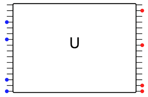
Noisy sampler
We present here the current best known approximate sampler, based on truncating probabilities in k perfectly interfering bosons and n-k perfectly distinguishable ones, an algorithm from https://arxiv.org/pdf/1907.00022.pdf. This decomposition is successful when some partial distinguishability is present. By simplicity, we restrict to the colloquial model of a one parameter x describing the overlap between two different photons (assumed to be equal for all pairs), which is implemented with OneParameterInterpolation. Similarly, loss is also accounted for.
Let us now explain the usage of this algorithm. As before, one creates an input of particles that are not completely indistinguishable from OneParameterInterpolation
julia> my_distinguishability_param = 0.7;

julia> my_mode_occupation = ModeOccupation(random_occupancy(n,m));

julia> my_input = Input{OneParameterInterpolation}(my_mode_occupation, my_distinguishability_param);
and still using my_interf with some loss η=0.7, one simulates our noisy boson sampling experiment with
julia> res = noisy_sampler(input=my_input, reflectivity=η, interf=my_interf)
3-element Vector{Int64}:
 5
 7
 11
where we have lost one particle as length(res)=3, meaning that only three output modes are populated by one photon.
Classical sampler
Finally, we repeat the steps to simulate fully distinguishable particles by using classical_sampler
julia> my_mode_occupation = ModeOccupation(random_occupancy(n,m));

julia> my_input = Input{Distinguishable}(my_mode_occupation);

julia> my_interf = RandHaar(m);

julia> res = classical_sampler(input=my_input, interf=my_interf)
 16-element Vector{Int64}:
 0
 0
 0
 1
 ⋮
 0
 1
 0